Previous Data Release from Summer 2012 [2]
2 SDSS Stripe 82 Reprocessing (co-adds and forced photometry)
LSST Data Management have recently finished building r-band SDSS Stripe 82 co-adds and performing forced photometry on individual epochs of g, r, and i-band Stripe 82 data.
The primary goal of this effort was to add the capability to make background matched co-adds to the DM stack, and test it at large scale by reprocessing real survey data. The full description of the challenge is available in the Winter 2013 Data Challenge Handbook.
Background matched co-adds preserve the diffuse astrophysical backgrounds in the stacked image. This increases its scientific usefulness. Furthermore, the thus constructed background in the co-add has higher S/N, making it easier to subtract it when needed. We plan to use this method to generate the co-adds in LSST production, and it was therefore important to have it built into the stack early. This will make upcoming tests of stackfit/multifit algorithms more realistic.
Our preliminary analysis indicates the quality of this dataset is comparable to the quality of Stripe 82 reprocessing we performed for Summer 2012, but with significantly more area. Nevertheless, we caution you that these data were processed “on a budget”, with prototype code, and minimal quality assessment. They are a byproduct of an ongoing software development effort, and not a result of a concerted scientific investigation. The code is still incomplete both in terms of features and quality, and the same will be true of the reprocessed data. In particular, if you plan to use this data set for science, expect to have to devote time to perform additional QA, and to have to communicate with DM developers to understand the details of the dataset.
If you do notice issues, or have questions, please don’t hesitate to contact us at <dm-help --at-- lsst.org>.
3 Data Access Rules
The data products provided by LSST DM are intended only for members of the LSST Science Collaborations unless noted otherwise. If their use results in a publication, their users will have to to abide by the LSST Publication Policy. [4]
The products are protected by a “well known” username and password: lsst / 3gigapix! .
Using this combination to access the data implies you understand and accept the restrictions on their redistribution and usage.
4 Data Locations
Note #1: Some of these websites require the standard DM user name and password; see the 3 Data Access Rules section for more information.
Note #2: The catalog and image access tools in use here are temporary solutions for data distribution built with off-the-shelf open source components: in particular, they are NOT representative of the Science User Interface the LSST will ultimately have.
Where to get data/information:
- Contact by email:
<dm-help --at-- lsst.org> - Winter 2013 Data Challenge Handbook.
- Catalogs access (phpMyAdmin): https://lsst-web.ncsa.illinois.edu/mydb/
- Note #1: if you don’t have a DM mysql database account, use this link to sign up.
- Note #2: You will need the “well known” username/password to access the signup form and the database entry page (see the 3 Data Access Rules section above).
- Note #3: If you’re accessing using the native mysql client, the database name is
DC_W13_Stripe82.
- FITS image access (coadds): See 4.1 Accessing Winter 2013 Coadd FITS Files.
- Co-add visualization tool: http://moe.astro.washington.edu/sdss/
- Data Management Software v6_1 Release (an intermediate Winter 2013 release).
If you decide to make use of this data, feel free to inquire about the details at <dm-help --at-- lsst.org>.
4.1 Accessing Winter 2013 Coadd FITS Files
The server lsst-web.ncsa.illinois.edu provides access to the data.
The entire namespace can be explored by pointing your browser to: http://lsst-web.ncsa.illinois.edu/lsstdata
The individual FITS files are stored in a directory hierarchy using the following scheme:
http://lsst-web.ncsa.illinois.edu/lsstdata/dr-w2013/deepCoadd/[ugriz]/<tract>/<patch>/coadd-[ugriz]-<tract>-<patch>.fits
where
[ugriz]is a single filter id from the indicated list (currently onlyr)<tract>is the LSST skymap tract id (currently 0 or 3)<patch>is the LSST skymap patch id (of the formxxx,yyy)
For example:
wget http://lsst-web.ncsa.illinois.edu/lsstdata/dr-w2013/deepCoadd/r/3/7,2/coadd-r-3-7,2.fits
Individual coadd files are 40MB (uncompressed).
5 Description of Data Products
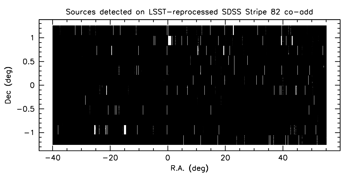
We used 298 runs imaged as a part of SDSS Stripe 82 (2 million fields) to create a deep co-add approximately covering -40 deg < R.A. < 55 deg, -1.25 < Dec < 1.25 (237 deg^2^).
No PSF matching was performed on the co-adds, making them deeper but less suitable for photometry.
The co-adds were used to detect 14.7 million sources, most of which would otherwise fall below the faint limit of individual exposures.
Photometry was performed in individual epochs, at the location of each source detected in the co-adds, resulting in 3.9 billion g, r and i band measurements (“forced photometry”).
u and z bands were not processed. We also produced catalogs of averaged forced photometry, both across the duration of the whole survey (~10 years), and on a yearly basis.
The co-adds are available as a series of 5126 FITS images, each spanning 2060 x 1937 pixels (see [wiki:W2013WebDataAccess] for how to access them). The catalogs are kept in a MySQL database and available through phpMyAdmin web interface, or (for power users), through the command-line mysql client. See the 4 Data Locations for instructions on how to access the database, and how to open an account if you don’t already have one.
The database contains 20 tables and views; however, only a few are of general interest (listed below). We do not have at this time a detailed description of the schema of each of these tables; however, the Summer2012 schema should provide sufficient information to understand the meaning of most of these columns even though the exact names may have changed.
Most frequently used tables:
| Column | Description |
|---|---|
| deepSourceId | object identifier |
| ra | Right Ascension (degrees) |
| decl | Declination (degrees) |
| nMag_[gri] | number of measurements for the band |
| magFaint_[gri] | magnitude of the faintest measurement in the band |
| medMag_[gri] | magnitude of the median measurement in the band |
| magBright_[gri] | magnitude of the brightest measurement in the band |
| q1Mag_[gri] | magnitude of the first (faintest) quartile measurement in the band |
| q3Mag_[gri] | magnitude of the third (brightest) quartile measurement in the band |
| faint5perMag_[gri] | 5th percentile magnitude in the band |
| bright5perMag_[gri] | 95th percentile magnitude in the band |
- AvgForcedPhot
- A table with percentiles of photometry in each band (5th, 25th, 50th (median), 75th, 95th). Columns are specified in the table above. All percentiles were calculated on the fluxes and converted back to magnitude for convenience.
- AvgForcedPhotYearly
- Same as the AvgForcedPhot table, except the percentiles are computed for each year of the survey. Therefore there are typically ~10 rows per object. Compared to AvgForcedPhot, this table has one extra column (‘’year’‘, running from 1 to 10), and no 5th and 95th percentile columns.
- DeepForcedSource
- Table with forced photometry measurements in individual epochs. Use this table if you’re interested in querying for complete light curves.
- DeepSource
- A table of sources detected on co-adds. This is in effect the master “object catalog”. Note however that because the co-adds were not PSF-matched, the photometry in this table will be relatively poor; use AvgForcedPhot table instead.
- RefObject
- A containing SDSS DR7 Stripe82 co-add [5] catalog. It’s been matched to DeepSource via RefDeepSrcMatch table.
- Science_Ccd_Exposure
- A table with metadata for all SDSS Stripe82 fields.
- Science_Ccd_Exposure_coadd_r
- A table with metadata for all co-add “patches” (when producing the co-add, we divided the sky into large “tracts”, and each tract has been subdivided into “patches”). The patches are stored as FITS files on the image server (see 4.1 Accessing Winter 2013 Coadd FITS Files).
6 Example Queries
Retrieve median g, r, i magnitudes for all objects in a (ra, dec) box:
SELECT
          ra, decl,
          medMag_g, medMag_r, medMag_i
FROM
          `AvgForcedPhot`
WHERE
                ra BETWEEN 0.01 and 0.02
        AND decl BETWEEN 0.03 and 0.04
Alternatively, you can use scisql geometry functions; this should speed up queries over large area:
SET @poly = scisql_s2CPolyToBin(0.01, 0.03, 0.02, 0.03, 0.03, 0.04, 0.01, 0.04);
CALL scisql.scisql_s2CPolyRegion(@poly, 20);

SELECT
        ra, decl,
        medMag_g, medMag_r, medMag_i
FROM
        `AvgForcedPhot`
WHERE
        scisql_s2PtInCPoly(ra, decl, @poly) = 1
Retrieve a g-band light curve for object 1398579058966639:
SELECT
    deepSourceId,
    deepForcedSourceId,
    exp.run,
    fsrc.timeMid,
    scisql_dnToAbMag(fsrc.psfFlux, exp.fluxMag0) as g,
    scisql_dnToAbMagSigma(fsrc.psfFlux, fsrc.psfFluxSigma, exp.fluxMag0, exp.fluxMag0Sigma) as gErr
FROM
    DeepForcedSource AS fsrc,
    Science_Ccd_Exposure AS exp
WHERE
        exp.scienceCcdExposureId = fsrc.scienceCcdExposureId
    AND fsrc.filterId = 1
    AND NOT (fsrc.flagPixEdge     | fsrc.flagPixSaturAny |
             fsrc.flagPixSaturCen | fsrc.flagBadApFlux   |
             fsrc.flagBadPsfFlux)
    AND deepSourceId = 1398579058966639
ORDER BY
    fsrc.timeMid
Notes:
- The times (timeMid column) denote the mid-points of exposure each SDSS frame. Since SDSS took data in TDI mode, these have to be corrected to the effective time of observation of each object.
- No effort has been made to remove objects doubly-detected in overlap regions of SDSS frames. You may therefore get more than one measurement per run.
Retrieve a g-band light curves for all objects with 0.0 < ra < 0.01deg and 0.0 < dec < 0.01deg:
SELECT
    deepSourceId,
    deepForcedSourceId,
    exp.run,
    fsrc.ra,
    fsrc.decl,
    fsrc.timeMid,
    scisql_dnToAbMag(fsrc.psfFlux, exp.fluxMag0) as g,
    scisql_dnToAbMagSigma(fsrc.psfFlux, fsrc.psfFluxSigma, exp.fluxMag0, exp.fluxMag0Sigma) as gErr
FROM
    DeepForcedSource AS fsrc,
    Science_Ccd_Exposure AS exp
WHERE
        exp.scienceCcdExposureId = fsrc.scienceCcdExposureId
    AND fsrc.filterId = 1
    AND NOT (fsrc.flagPixEdge     | fsrc.flagPixSaturAny |
             fsrc.flagPixSaturCen | fsrc.flagBadApFlux   |
             fsrc.flagBadPsfFlux)
    AND fsrc.ra BETWEEN 0.0 AND 0.01
    AND fsrc.decl BETWEEN 0.0 AND 0.01
ORDER BY
    fsrc.deepSourceId, fsrc.timeMid
Notes:
- Expect this query to take 1-2 minutes to complete. It will return 2,014 rows.
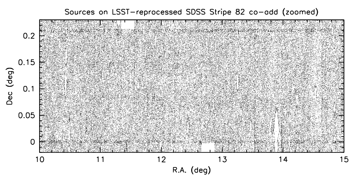
7 Covered footprint
A quick visualization of the footprint available in Winter 2013 Stripe 82 data, created by plotting all 15.9 million detected objects:
8 RGB Color composites
RGB color composite of an area in the vicinity of M2:
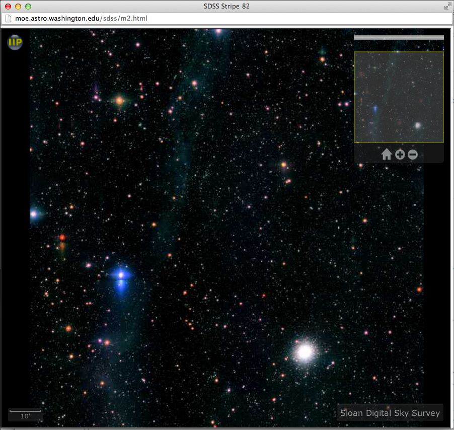
The full-sized image can be viewed/panned/zoomed at http://moe.astro.washington.edu/sdss/.
9 Quality assessment
9.1 Comparison to S2012 and Completeness
We took a small subset of data from both the Summer 2012 DC and the Winter 2013 early production DC. Using the DEEP2 catalogs [6] as reference, we compare the completeness as a function of magnitude between the two reductions.
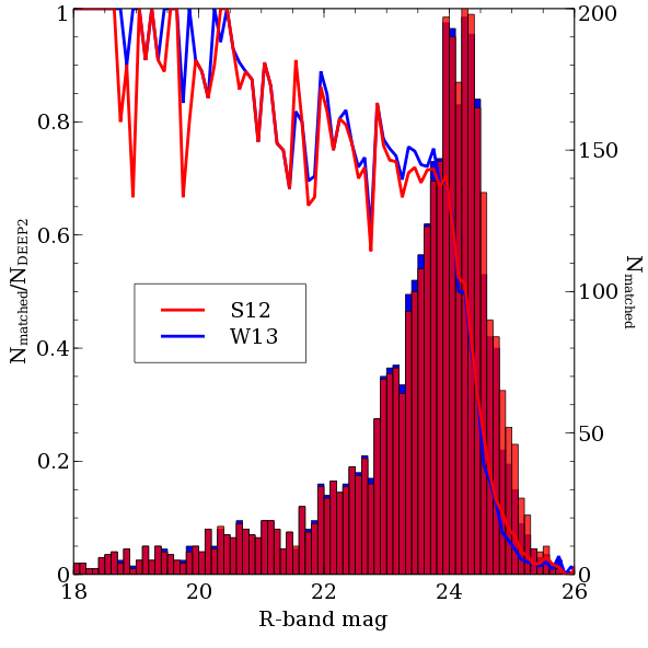
The Winter 2013 (blue) completeness tracks very well with the Summer 2012 (red). This shows that we have not changed anything substantial between the two reduction runs.
We next look at a much large section of the survey covering the Deep2 Field 4 photometric catalogs. We construct completeness and contamination profiles for the Winter 2013 DC.
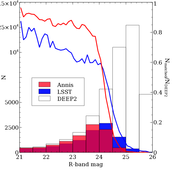
In addition to comparing to the DEEP2 catalogs, we compare the completeness of the Annis (2014) [5] catalogs to the Winter 2013 results. The Winter 2013 catalog is significantly less complete at bright magnitudes. We are looking more into this, but early evidence suggests this is due primarily to background subtraction around bright stars and to the fact that multiple peaks within a single detection footprint are not de-blended into individual sources for the Winter 2013 runs. We have placed a 5-sigma S/N threshold on the Annis catalog and the Winter 2013 catalog does not go significantly below 5-sigma. With these cuts the Winter 2013 catalog goes ~0.2 mag deeper than the Annis catalog.
The completeness plot is not the whole story. We also look at the trends in S/N between the Annis (2014) [5] catalog and the Winter 2013 catalog.
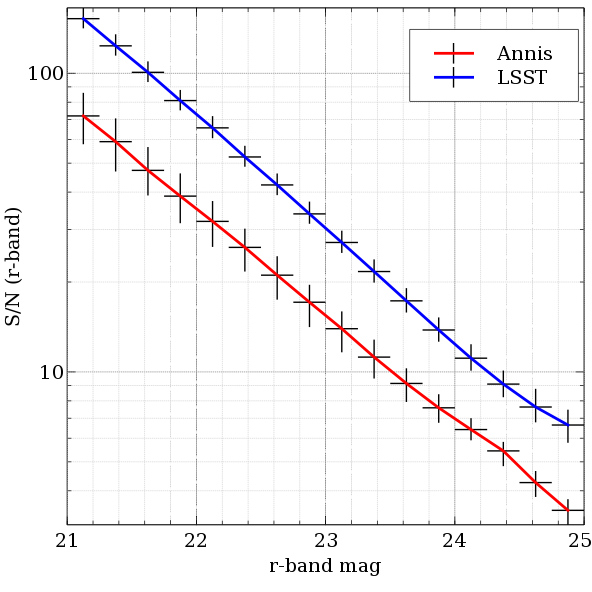
This shows that for constant S/N the Winter 2013 catalog goes about 0.75 mag deeper than the Annis (2014) [5] catalog. We also see that the Winter 2013 catalog is 10-sigma at our 50% limiting magnitude of 24.2. This suggests that a 5-sigma threshold on the coadd to seed forced photometry is too conservative and that we should have pushed to 3-sigma (or fainter) in the coadd to reach completeness in the coadded catalog at 5-sigma.
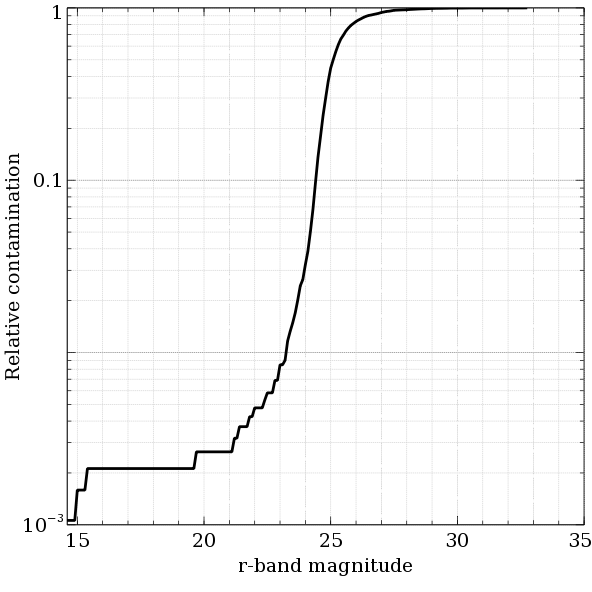
We also looked for contamination in the Winter 2013 catalog. We define contamination simply as any object in the Winter 2013 catalog that is not in the DEEP2 catalog. The following figure shows that there is less than 5% relative contamination to our limiting magnitude.
The production pipelines perform photometric calibration using the catalog of Ivezic (2007) [8]. In this analysis we look at the distribution of forced photometry principal colors of stellar sources, described in Ivezic (2004) [7]. We use the star-galaxy separation provided by the Annis (2014) [5] Stripe82 catalog to select point sources for the analysis; we do not do any native star-galaxy separation. The figure below illustrates the process of defining a principal color (adopted from Ivezic (2004) [7]):
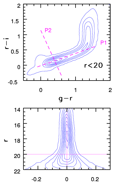
The width of the stellar locus perpendicular to principal color P1 (top) is a function of underlying stellar astrophysics, and errors on the photometry.
As the bottom panel demonstrates, this width increases as a function of magnitude, as photometric uncertainties start to dominate.
In our analysis, we look at the principal colors w, shown in the figure above, and x, which is the width perpendicular to the vertical distribution in the (r-i) vs. (g-r) diagram above.
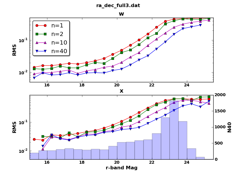
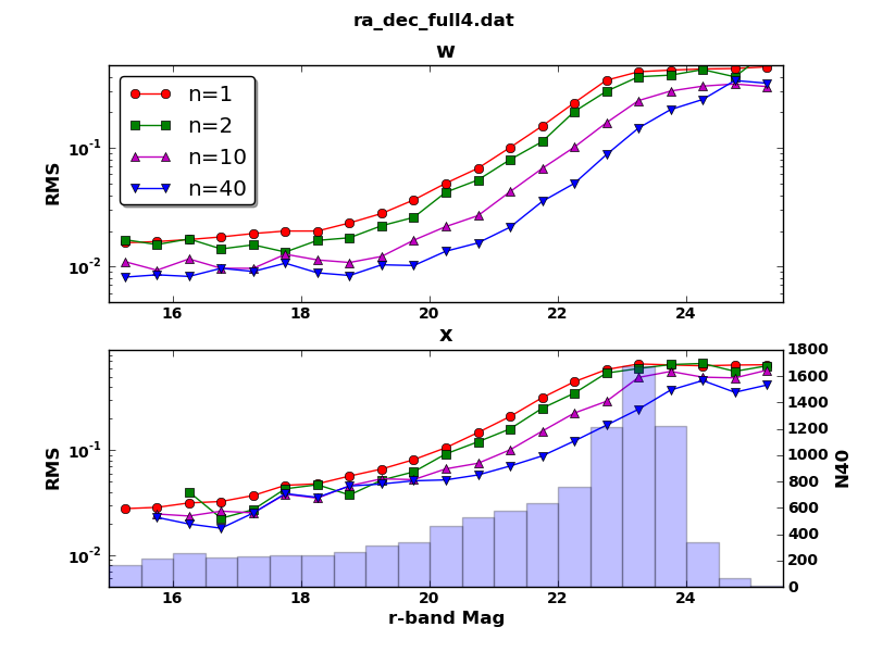
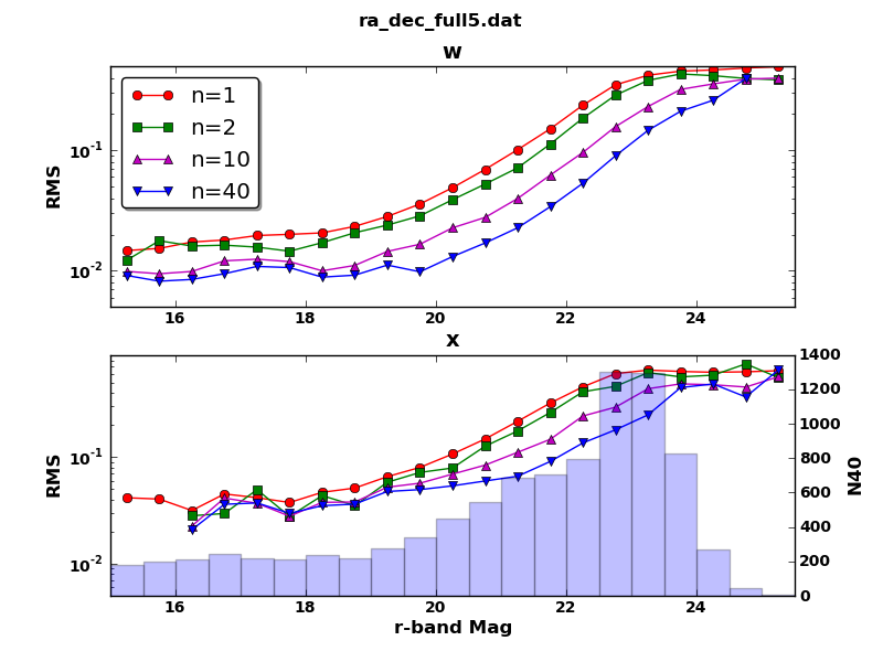
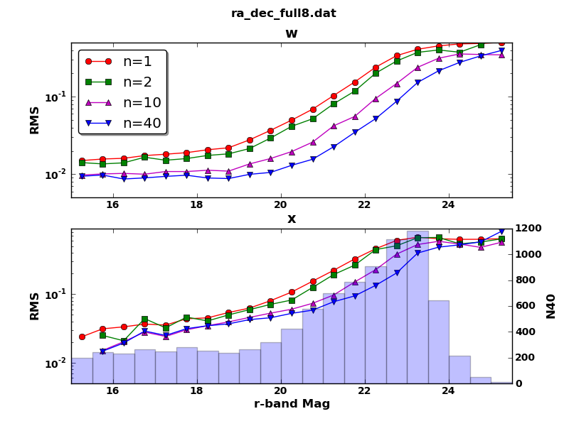
We examine below the width of the principal loci as a function of the number of epochs for forced photometry: using 1 epoch (i.e. all the data), the median (in flux) of two epochs (where the flux medians to a value > 0.0), and the median of 10 and then 40 epochs.
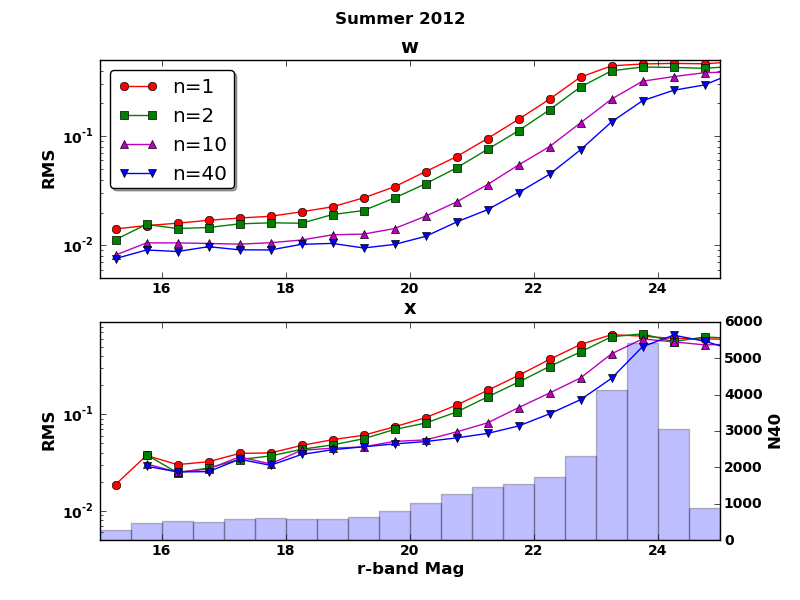
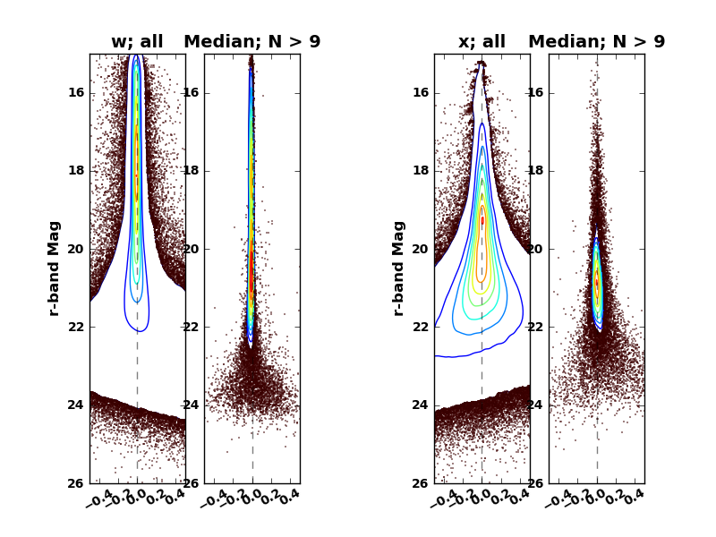
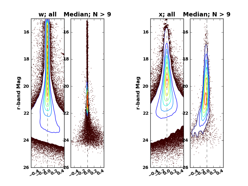
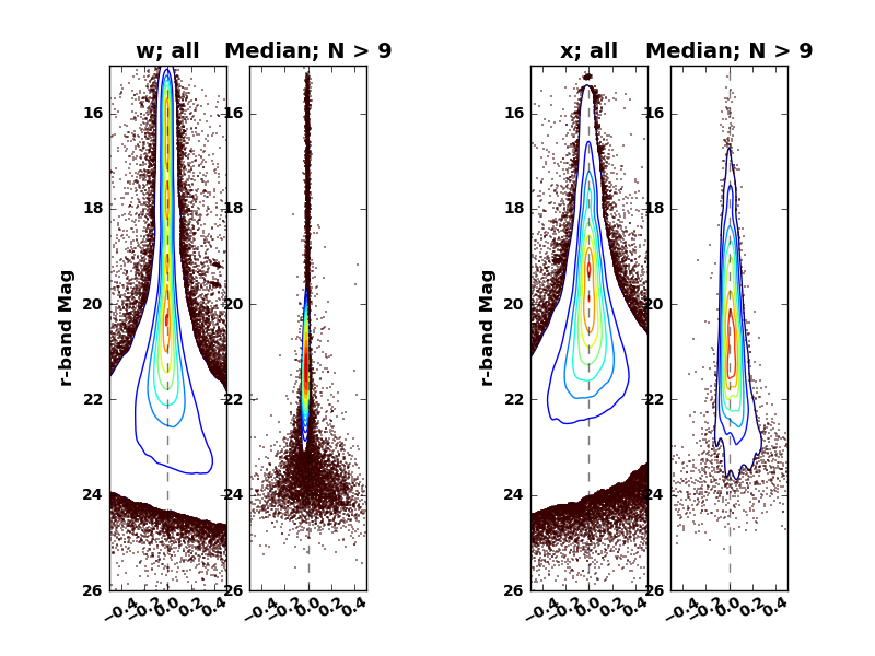
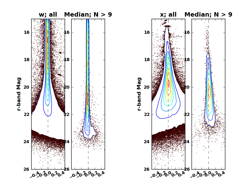
We first show the results for Summer2012 processing below:
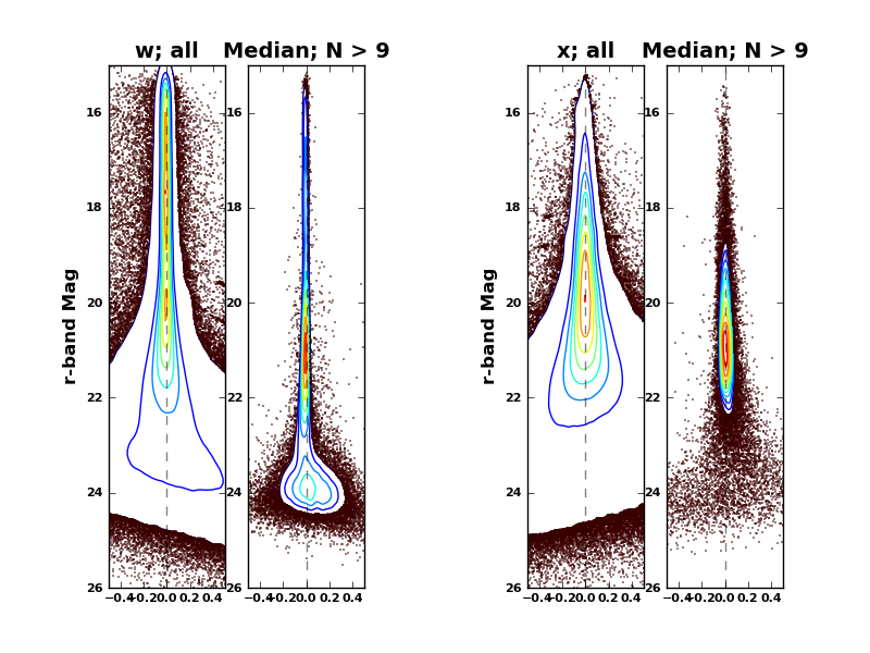
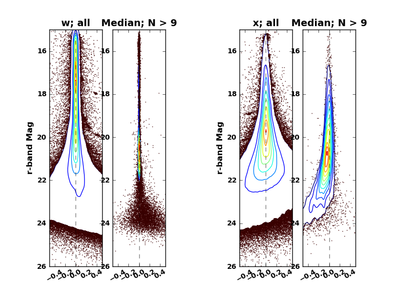
The left image provides the distribution of points around the principal colors w and x (i.e. the principal locus is at x=0 in all plots).
Each panel shows the all-data distribution, and then the median across epochs for all objects with N>9 epochs. When medianing across many measurements, the locus becomes tighter, and is less dominated by the photometric uncertainties to fainter magnitudes.
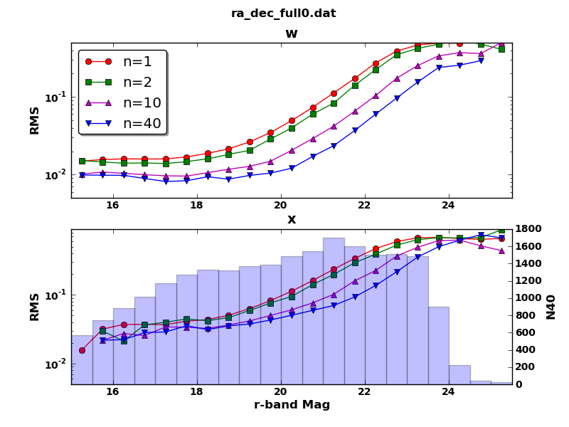
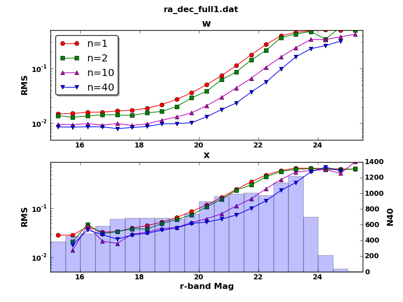
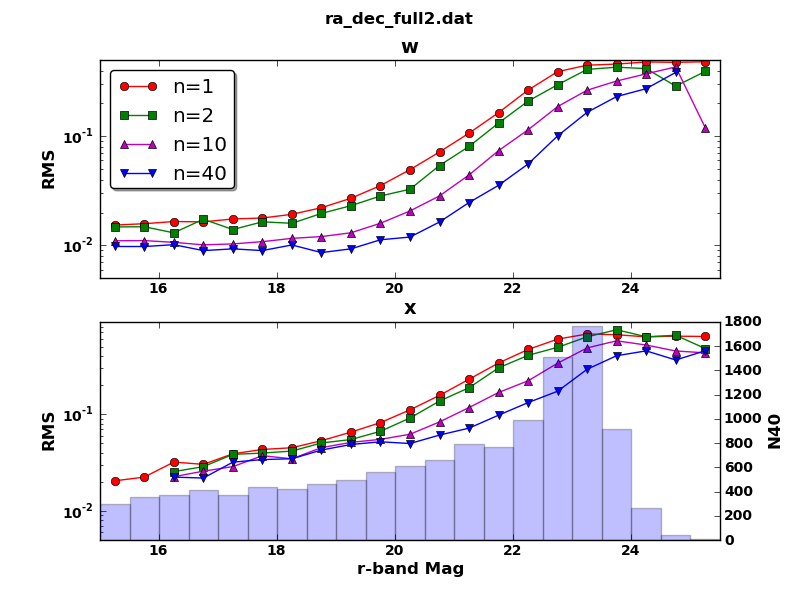
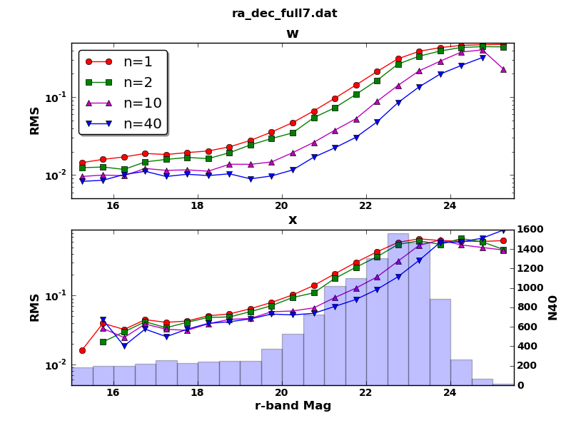
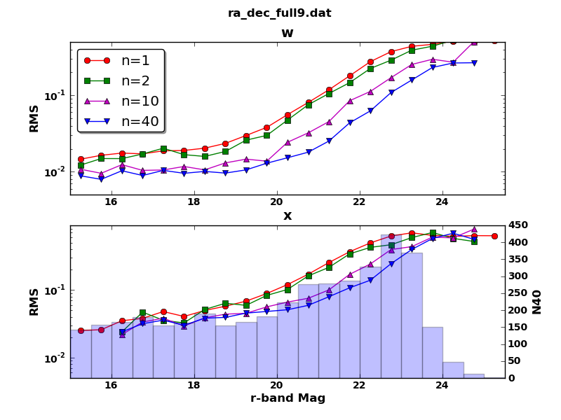
The right panel shows how the width of this locus improves as a function of the number of epochs, for N=1,2,10,40 epochs, along with a histogram of the number of objects vs. r-band magnitude.
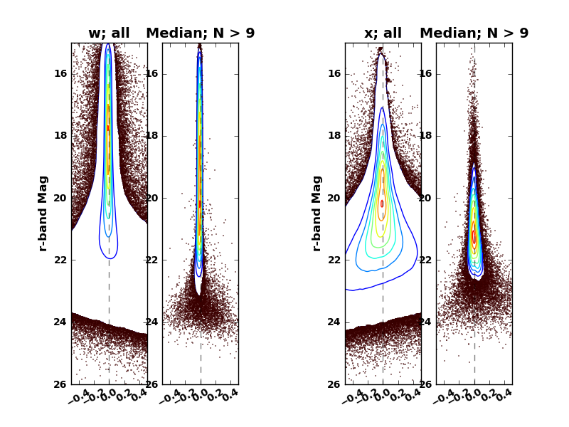
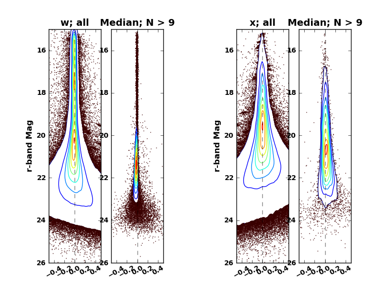
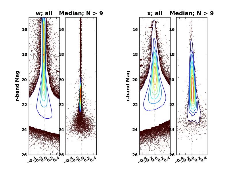
We examine below the results of the Winter2013 processing for one of the 6 SDSS camcols. This includes data from camcol=1 of both the N and S strips of the stripe. We subdivide the data into areas 10 degrees wide in RA, and provide measurements of the median and standard deviation of the distributions (computed as 0.741 times the interquartile range) in tabular form for the first RA range.
9.1.1 -40 < RA < -30
Mag             w;N=1        w;N=2       w;N=10       w;N=40                             x;N=1        x;N=2       x;N=10       x;N=40
15.25      -0.004,0.015 -0.006,0.015 -0.002,0.010 -0.002,0.010                      -0.027,0.016      ...          ...          ...
15.75      -0.004,0.016 -0.003,0.015 -0.003,0.011 -0.003,0.010                      -0.009,0.032 -0.008,0.030 -0.010,0.022 -0.006,0.022
16.25      -0.003,0.016 -0.002,0.014 -0.002,0.010 -0.002,0.010                      -0.015,0.037 -0.006,0.021 -0.013,0.027 -0.009,0.022
16.75      -0.003,0.016 -0.004,0.014 -0.003,0.010 -0.002,0.009                      -0.016,0.037 -0.015,0.036 -0.019,0.026 -0.018,0.028
17.25      -0.003,0.016 -0.003,0.014 -0.002,0.010 -0.002,0.008                      -0.007,0.037 -0.007,0.040 -0.005,0.034 -0.004,0.029
17.75      -0.002,0.017 -0.001,0.015 -0.002,0.010 -0.002,0.008                       0.001,0.041 -0.008,0.044  0.002,0.034  0.004,0.035
18.25      -0.002,0.019 -0.002,0.016 -0.002,0.011 -0.002,0.009                      -0.003,0.044 -0.007,0.042  0.001,0.032  0.000,0.031
18.75      -0.002,0.021 -0.003,0.018 -0.001,0.012 -0.001,0.009                       0.000,0.050  0.001,0.047  0.002,0.036  0.002,0.035
19.25      -0.002,0.026 -0.002,0.021 -0.002,0.013 -0.002,0.010                       0.004,0.063  0.005,0.059  0.004,0.042  0.006,0.038
19.75      -0.002,0.035 -0.003,0.029 -0.001,0.015 -0.002,0.010                      -0.000,0.082 -0.000,0.076  0.001,0.050 -0.000,0.043
20.25      -0.002,0.050 -0.003,0.040 -0.002,0.021 -0.002,0.012                       0.003,0.112  0.011,0.094  0.005,0.060  0.003,0.050
20.75      -0.002,0.074 -0.003,0.060 -0.003,0.029 -0.003,0.017                       0.003,0.161  0.001,0.140  0.006,0.076  0.003,0.059
21.25      -0.001,0.113 -0.008,0.083 -0.005,0.042 -0.006,0.024                       0.005,0.234  0.003,0.197  0.009,0.101  0.007,0.070
21.75       0.017,0.173  0.007,0.141 -0.008,0.066 -0.007,0.037                      -0.008,0.337  0.004,0.291  0.015,0.159  0.017,0.093
22.25       0.056,0.274  0.043,0.225 -0.008,0.104 -0.012,0.060                      -0.044,0.466 -0.034,0.388  0.033,0.225  0.034,0.136
22.75       0.128,0.390  0.081,0.350 -0.000,0.174 -0.011,0.097                      -0.176,0.591 -0.096,0.525  0.064,0.364  0.064,0.215
23.25       0.249,0.467  0.178,0.422  0.035,0.254  0.005,0.155                      -0.403,0.672 -0.309,0.631 -0.019,0.490  0.095,0.352
23.75       0.470,0.495  0.361,0.478  0.138,0.338  0.043,0.240                      -0.722,0.681 -0.625,0.674 -0.275,0.610  0.026,0.499
24.25       0.780,0.493  0.632,0.549  0.372,0.372  0.145,0.257                      -1.058,0.654 -0.985,0.668 -0.641,0.621 -0.179,0.618
24.75       1.112,0.514  0.934,0.480  0.673,0.362  0.437,0.293                      -1.400,0.637 -1.169,0.675 -1.064,0.514 -0.597,0.743
25.25       1.448,0.525  1.299,0.411  0.963,0.503      ...                          -1.742,0.659 -1.615,0.879 -1.434,0.437 -1.155,0.668


10 References
| [1] | Andrew Becker and others. Report on Late Winter2013 Production: Image Differencing. LSST Data Management LDM-227, 2013. URL: https://ls.st/LDM-227. |
| [2] | Mario Juric. Summer 2012 LSST DM Data Challenge. LSST Data Management Tech Note DMTN-0034, 2012. URL: https://dmtn-034.lsst.io. |
| [3] | Richard A. Shaw and others. LSST Data Challenge Report: Summer 2012/early-Winter 2013. LSST Data Management LDM-226, 2013. URL: https://ls.st/LDM-226. |
| [4] | Project Science Team. LSST Project Publication Policy. LSST Data Management LPM-162, 2015. URL: https://ls.st/LPM-162. |
| [5] | (1, 2, 3, 4, 5) J. Annis and others. The Sloan Digital Sky Survey Coadd: 275 deg^2 of Deep Sloan Digital Sky Survey Imaging on Stripe 82. ApJ, 794:120, October 2014. arXiv:1111.6619, doi:10.1088/0004-637X/794/2/120. |
| [6] | A. L. Coil, J. A. Newman, N. Kaiser, M. Davis, C.-P. Ma, D. D. Kocevski, and D. C. Koo. Evolution and Color Dependence of the Galaxy Angular Correlation Function: 350,000 Galaxies in 5 Square Degrees. ApJ, 617:765–781, December 2004. arXiv:astro-ph/0403423, doi:10.1086/425676. |
| [7] | (1, 2) Ž. Ivezić and others. SDSS data management and photometric quality assessment. Astronomische Nachrichten, 325:583–589, October 2004. arXiv:astro-ph/0410195, doi:10.1002/asna.200410285. |
| [8] | Ž. Ivezić and others. Sloan Digital Sky Survey Standard Star Catalog for Stripe 82: The Dawn of Industrial 1 per cent Optical Photometry. AJ, 134:973–998, September 2007. arXiv:astro-ph/0703157, doi:10.1086/519976. |
Note
This document was originally published as an LSST TRAC page at https://dev.lsstcorp.org/trac/wiki/DC/Winter2013